• Applied Algorithms Series
• 0: Image Sort
  • 1: Problem Analysis
    • 1.1: Algorithms: Sort
    • 1.2: Data Structures: Image
  • 2: Solution
  • 3: Algorithm
    • 3.1: How it Works
    • 3.2: Image and Sorting
  • 4: Implementation
    • 4.1: How To Read
    • 4.2: Objective
    • 4.3: Code
      • 4.3.1: Create a Data Structure
      • 4.3.2: Open an Image
      • 4.3.3: Vectorize
      • 4.3.4: Sort
      • 4.3.5: Construct a New Image
      • 4.3.6: Save a New Image
      • 4.3.7: Form a Program
  • 5: Outcome
    • 5.1: Input and Output
  • 6: Result Analysis
  • 7: Further Development

Applied Algorithms Series

This is the first post in a blog, and this is the first post in Applied Algorithms series. This series will be about algorithms and their applications, or to rephrase it, this series is about various problems and how to solve them using algorithms.

The main emphasis will be on a problem analysis and implemented in code solution. Each article will have a fully working code project. Implementation language of choice will be the most suitable one for a problem. For some problems, it will be C++, for other problems Python, and perhaps some other languages if they fit the problem well.

Algorithms in books, such as CLRS, lacks creativity, which is natural for that kind of books, however, this fact somewhat annoys me, because I think that algorithms are a highly creative topic and their application could be quite interesting and intriguing. While I personally find mathematics beautiful, some people may experience some different feelings about it. For these people, I want to show the bright side of algorithms. For those who love mathematical side of algorithms, I want to show an applied side of them.

The main purpose of this series is a casual education for some people, and a pleasant computer science read for the other. Because the target audience is somewhat wide, in the first post of the series I will write about some basic things too, and in latter articles, I will point on the older posts. If you do not understand something - that’s fine, just read further. If something is too clear to you skip to another paragraph, hopefully, it will get more interesting.

I often mix code notation and $ math $ notation. I do this with a reason. In articles you will see some formulas and math explanations because some concepts are purely mathematical, and therefore should be expressed in mathematical language. However, I try to express each idea such that everyone will understand it. I explain each formula explicitly. I know that every math expression reduces audience, but I think that computer science and mathematics are always going hand-by-hand, and, after all, math is not that scary as people tend to think.

0: Image Sort

Imagine a problem: you need to sort an image. Yes, literally, pixel-wise. Before approaching any problem, one should figure out the nature of the problem and related entities. This strategy can be found not only in computer science but in every field where you need to solve something “big”. Even most complicated task boils down to an atomic procedures, where the atomic procedure is an abstract concept of a minimal possible step. And yes, while atom is not indivisible anymore, we will stick to that mnemonic convention.

1: Problem Analysis

Our problem, an image sort, is made out of two parts/concepts:

1. Sort
2. Image

Essentially, these two parts can be generalized into two topics: algorithms, and data structures. Sorting is a problem of algorithms, while an image is the problem of data structures.

1.1: Algorithms: Sort

While we are speaking about algorithms we often mean efficiency. It is easy to understand algorithms importance on the following statement:

Algorithms make previously impossible task possible.

The difference is not only between few milliseconds but between possible and impossible.

Next, when we are talking about algorithms (efficiency) we usually concerned about their time, and sometimes, space complexities, because computer science, unlike theoretical mathematics, is dealing with reality, and reality always introduces some physical constraints.

On wikipedia one can find a plenty of sorting algorithms. There are two kinds of sorting algorithms:

1. Comparison sort algorithms
2. Non-comparison sort algorithms

The main difference between them in that comparison sorts can not perform better than O(n log(n)).

A little spoiler here, we will sort an image in $ \mathcal{O}(n) $ time, which is quite a good result.

The natural question is: “What algorithm should we prefer?”. To answer this question we must understand a nature of data, or an input of our algorithm.

1.2: Data Structures: Image

When I said that images belong to data structures it was only a half of the truth, because most image formats are actually algorithms too. Compression algorithms to be precise. If you are feeling curious about compression stay tuned, I’m planning to write a similar kind of an article about compressions with plenty of examples.

However, besides compression, images are data structures, and now we are going to dig into them.

Black and white image of w pixels wide and h pixels height represented in a computer memory as a matrix X where h corresponds to rows, and w to columns. While there is no such a thing as a matrix primitive in a common computer, we still can say “in a computer memory” because the matrix is an abstract data type.

Let’s take 3x3 grayscale image. 3 pixels wide, 3 pixels height. Each pixel value corresponds to a brightness. The pixel of value 0 is 0% bright, while pixel of value 255 is 100% bright. Pixels values ranges in 0..(2^8)-1 or 0..255. 0..255 range takes 1 byte of space because any value from 0 to 255 can be represented using 8 bits.

3x3 matrix correspond to 3x3 image:

The Very same idea goes for RGB images, but instead of 1 matrix, we have 3 matrices. For example 3x3 RGB image will represented in memory as three 3x3 matrices: R, G, B.

To form an image these three matrices, R, G, B, are layered:

As with black and write images, in colored each pixel represents a brightness. Value of 255 in the R matrix and 0 in G and B will yield a purely red color. Same values at the same positions in all three matrices positions will yield some black-and-whitish color.

Here is some helpful notation. How would you represent a bottom middle pixel, which is greenish one? Matrices usually named with capital letters, such as $ A $, and they have dimensions. $ m $ stands for rows, and $ n $ stands by columns. This looks like so in math notation $ A^{m \ \times \ n} $, or better to say that matrix $ A $ belongs to some $ m \ \times \ n $ space:

$$ A \in \mathbb{N}^{3 \times 3} \ | 0 <= a_{i, j} <= 255 $$

This expression states that: matrix $ A $ belongs to a natural number space of $ 3 \times 3 $ dimension, and each element of this matrix are in the range of 0 .. 255.

Now we have the instrument to point at a particular element, pixel, in our matrix.

Therefore, $ r_{3,3} = 255, g_{3,3} = 45, b_{3,3} = 4 $ form a redish pixel in the image’s right bottom corner. Note that a lowercase letter implies element of a matrix, while uppercase refers to a maxtrix itself.

For an intuition model, you can imagine image pixels as vectors on some planar space, a surface. This surface is a visible image, and each of these columns represents a single pixel:

Now we are at the point where we are able to draw some conclusion. Image data structure is stable and fixed. For grayscale images, we have one matrix where rows equal to the height, columns to width. For RGB image we have three matrices with the same properties. All pixel values in the range of (2^8)-1 or `0..255. An atomic piece in an image is a pixel. While image formats may vary data container, a matrix, will always remain the same.

2: Solution

Now we have a good understanding of an underlying data structure, and now we should pick some sorting algorithm. As was mentioned previously there are two kinds of practical sorting algorithms (and three in general): comparison, and non-comparison. Also, we know that comparison sorts can not perform better than $ \mathcal{O}(n \log(n)) $.

Let’s combine these two pieces. Our data structure is stable and each data point is always in range of 0..255. And there is an algorithm which fits our data structure perfectly well: counting sort.

3: Algorithm

Counting sort is a stable, non-comparison algorithm, with $ \mathcal{O}(n + k) $ time complexity and $ \mathcal{O}(n + k) $ space complexity. In case if you aren’t familiar with $ \mathcal{O} $ notation, you may find this read useful. As we know from asymptotic analisys , we are concerned about asymptotical behavior, how an algorithm will perform over time with various inputs.

For example, if our algorithm behavior, where $ x $ is an input size, can be expressed as the following time function

$$ f(x) = x^2 + x $$

which for example might be something like these two blocks of code

def f(n):
    '''
    Possible version of x^2 + x function
    '''
    for i in range(n):
        for j in range(n):
            # some constant time thing

    for k in range(n):
        # another constant thing

f(n) is $ \mathcal{O}(n^2) $ anyway, despite that second loop over k. The short and not rigorous explanation for that fact is that we are interested in a growth rate, which is the highest degree of our $x$. This is because we want to predict algorithm’s behaviors, not to find its exact number of operations. Why? Well, we can not find an exact number of operations due to various factors such as a computer architecture or processor implementation details. All discussions about algorithms are implicitly based on random-access machine.

A quick quiz: What is a time complexity in $ \mathcal{O} $ (Big-oh) notation of the following function?

$$ f(x) = x^3 + x^2 * 8000 $$

If your answer is $ \mathcal{O} $ of $ n $ in third power – you got it right.

If no, think about it in this way: you have two $ x $ which can be any number which is bigger than zero (because how an algorithm is supposed to perform something with a negative input, and what does a negative input even mean), and one constant. Despite a huge constant and multiplication, $ x^3 $ matters more. Lets write a simple script to find sufficiently large $ x $ when $ x^3 $ overweight the rest:

def f(x):
    return (x**3, x**2 * 8000)

def find_overweight():
    counter = 1
    res = f(counter)
    while (res[0] < res[1]):
        print(res, counter)
        counter += 1
        res = f(counter)

After calling this function we will learn that when $ x = 8000 $ the two parts will be equal, which is clearly can be seen here: $ 8000^3 - 8000^2 * 8000 $ will yield $ 0 $. So, after $ x > 8000 $ $x$ is sufficiently large. How big is it? Well, it is approximately 52x51 RGB image. Not big at all. That’s why we are interested in the highest degree. Highest degree will always outweigh with a sufficiently large input.

Comming back to counting sort. Now you may have a reasonable question, why do we have $ n + k $ part in time and space complexities of counting sort, when we just learned that we care only about the highest power? The answer for this in the nature of counting sort.

3.1: How it Works

The algorithm takes an input array arr. We set $ n $ to be equal to arr’s length, and $ k $ to arr’s range, where the range is the maximum value stored in arr.

Next, the algorithm has two conceptual steps:

• Counting
• Sorting

During the counting part algorithm creates (allocates) additional array of length $ k $ and iterates, linearly, over each element in the input array. On each iteration algorithm increments value by one in the additional array at the index which corresponds to the value of an element from the input array at which iteration is currently set. In other words: it counts how many of each value in a given range the input array has.

During the sorting part algorithm goes through each index in the additional, or counting, array, and if a value at this index is not zero it writes this index as a value into the resulting array decrementing this value in the counting array. Repeat until value gets to zero.

Lets go step-by-step:

We have the input array of [2, 3, 3, 1, 1, 5, 1, 3, 4, 1], so our $ n = 10 $. Array has range of 5 because $ max(array) = 5 $, therefore $ k = 5 $. This is important, and why it is so I will explain later on a “bad” example.

Now we have input, counting, and output arrays. We go through each element in the input array and increment value in counting array at the index of value the current element. For example, 1st element in input is 2, therefore we increment value at counting[2] by one. Thus the name: counting sort. We basically just counting each element in the input array. That’s why we really need to know the range of values in the input array.

Counting sort is an elementary algorithm, yet quite powerful in a right use case. However, this use case is quite limited by input’s array data. If data has a small and predictable range then counting sort is a great solution.

Lets look what is the “bad” case looks like:

Our $ n = 4 $, $ k = 34829 $. This case is exact reason why time and space complexity of a counting sort is $ \mathcal{O}(n + k) $.

The problem is that in such case algorithm will allocate a counting array of length 34829 + 1 in order to sort 4 elements. If array has a type of int and int is 32 bits or 4 bytes, then this array will cost 139316 bytes of memory, instead of 16. Another problem is that sorting part of the algorithm goes through each element therefore instead of 4 operations algorithm will perform 34829 + 1, which is quite “bad”.

We can generalize this to rule such as: if $ n < k $ then, perhaps, counting sort is not the best possible solution.

3.2: Image and Sorting

Now we have all background and necessary knowledge to conclude that counting sort fits image data model very well. In images $ n $ value is much, much bigger than $ k $.For example screenshot from HDPI display of 2880x1800 pixels has $ n = 15552000 $ and $ k = 255 $.

Knowledge of $ n $ value also important because it could help or harm. For example, if $ n $ in range of $ {0, 1, …, 65535} $ we can use short int[k] as a counting array type and save some space (given that we are sure that short int is guaranteed to be at least 16 bits). Or if our $ n $ is in range of $ {0, 1, …, 2^{64} - 1} $ then we must use long long int[k]. The reason is that in an image we can not predict pixel distribution. For example, a compitely black image of size 32 x 32 pixels will have counting array of length 256, as any other counting array of image, but the first element in the counting array at index 0 will have the value of 1024 while other 255 indexes will store 0.

4: Implementation

4.1: How To Read

The language of choice here will be C++ because we want to have full control over our data structures and space. Because of this choice here is my recommendation how to read this part: I will write here code and algorithms, and discuss them. However, I will describe only interesting parts.

Here,

you can find a fully working project which you can git clone and make. Note that code has opencv2 dependency for working with image formats and containers.

Because C++ is harder than Python I used only basic language features such as raw pointers, not smart pointers, so that every person who coded at least in C will be able to understand whats going on.

4.2: Objective

Lets set a practical objective for our code. Our program should take path to an image as an input, and produce a sorted image as an output saving it in ./samples/ directory.

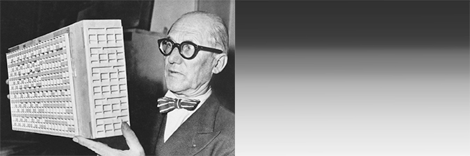
And let’s take an image:

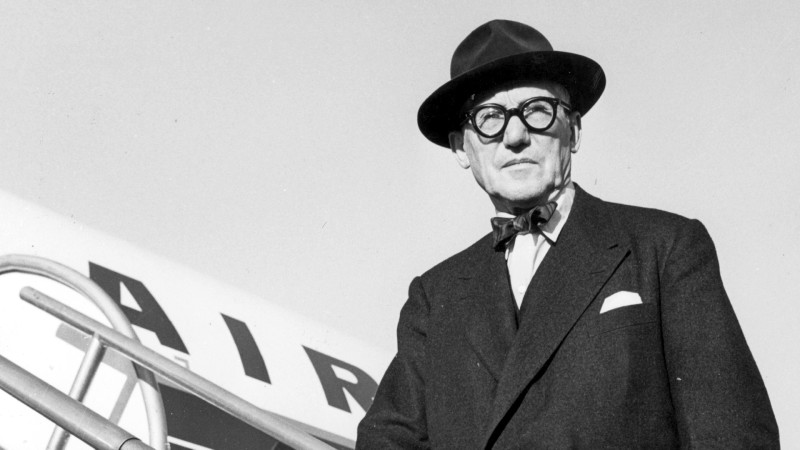
No, I am very sorry, it is not a cat picture. It is a photo of Le Corbusier, architect and basically one of the pioneers of the modern architecture. 1910 - 1930 was a golden era of a modern design, minimalism, conceptualism, but unfortunately due to more important world agenda achievements and discoveries of these years in architecture and design never was in a wide public focus.

Techical side of this image is:

$$ width = 800, height = 450, channel = 1, k = 255, n = 360000 $$

The following discussion will be based on this image and its values.

4.3: Code

First, let’s outline our strategy:

1. Create a data structure
2. Open an image
3. Vectorize
4. Sort
5. Construct a new image
6. Save a new image
7. Form a program

Each paragraph will have a link to implementation on GitHub in the last sentence because of some pieces will be omitted as irrelevant to the discussion, but relevant for a compiler. If it is happened to you to don’t know about classes, feel free to skip Create a Data Structure part and ignore Class::method syntax.

4.3.1: Create a Data Structure

We are working with an image, therefore we can abstract our image and underlying procedures, such as sorting, to a class.

class Image {
private:
    // Members
    cv::Mat mat;
    uint rows;
    uint cols;

public:
    // Constructors
    Image(cv::Mat&);
    Image(std::string);

    // Methods
    void open(std::string);
    void save(std::string);

    uint8_t* vectorize();

    uint get_rows() { return rows; };
    uint get_cols() { return cols; };

    // Static functions
    static cv::Mat  vector_to_mat(uint8_t*, int, int);
    static uint8_t* sort(uint8_t*, int, int);
}

We have three members which represent actual image data. While rows and cols are clear, cv::Mat needs some explanation. You can find it here in opencv documentation. TL;DR version is that cv::Mat is a matrix with some extra features. It stores image’s matrix, pixels.

Two class constructors, where Image(cv::Mat&) constructs an image from existing opencv matrix, and Image(std::string) constructs an image instance from a file which is provided in a string.

Methods and static functions will be discussed later.

4.3.2: Open an Image

Thanks to opencv library one can use cv::imread(path, kind) method to read an image from a given path straight into cv::Mat type.

Image::Image(std::string path) {
    if (path.empty())
        throw std::runtime_error("path error");
    
    mat = cv::imread(path, CV_LOAD_IMAGE_GRAYSCALE);

    if (!mat.data)
        throw std::runtime_error("no data error");

    rows = mat.rows;
    cols = mat.cols;
}

First if statement is a sanity check. If we have no path, no image can be opened. Here is one interesting point. If our path in an empty string, then cv::imread most likely will throw an exception, right? Well, most likely yes, but I found that it is a way easier to debug if you are throwing your own exceptions in your code. 3-rd party exceptions might be very cryptic to read and difficult to debug.

Next expression will read image’s content into mat member. If after that procedure mat has no data this is an exception for us too.

Also, we store a state of our rows and cols (columns) in a class instance.

4.3.3: Vectorize

Vectorization is a procedure, a linear transformation, which converts a matrix into a vector.

$$ A = \begin{bmatrix} a & b \\ c & d \end{bmatrix} $$

$$ vec(A) = \begin{bmatrix} a & b & c & d \end{bmatrix} $$

$ A $ matrix here is a valid representation of 2x2 pixel grayscale image. However, to sort it we need to convert it to something iterable. Vector is a perfect data representation for this task. Note that during vectorization we are losing the shape of an image. That’s why we store image’s shape in rows and cols.

uint8_t* Image::vectorize() {
    auto row_vector = new uint8_t[rows * cols];

    int index = 0;
    for (int i = 0; i < rows; i++) {
        for (int j = 0; j < cols; j++) {
            row_vector[index] = mat.at<uchar>(i, j);
            index += 1;
        }
    }

    return row_vector;
}

The return value has a type of a pointer to uint8_t. This type, as can be found in documentation is an unsigned integer type with the width of exactly 8 bits. This is exactly what we need, not more, not less. 8 bits can store 2^8 - 1, or 255 in decimal. -1 because there are 256 items in $ {0..255} $ set. To store 256 we already need 16 bits.

First, we allocate enough space to store all the pixels: rows * cols of uint8_t.

Next, we iterate over each row, and in each row we iterate over each column, writing element one-by-one into row_vector. In opencv element in matrix can be accessed as mat.at<uchar>(i, j).

For example:

$$ A = \begin{bmatrix} a & b \\ c & d \end{bmatrix} $$

will be transformed into the array of [a, b, c, d].

Therefore, after vectorization, we will get a row_vector, which is a simple plain C-style array.

What is about time complexity? One may say that time complexity is $ n^2 $ and will be wrong. Two nested for loops aren’t always mean $n$ square complexity. Our $ n $ is defined as 360000, and in our algorithm, we are visiting each element in each row. We have 450 rows and 800 columns. 450 * 800 is exactly 360000. Time complexity is $ \mathcal{O}(n) $, or better to say $ \theta(n) $. I won’t clarify this point because it is a topic for a separate, and quite a big, article.

Space complexity is also $ \mathcal{O}(n) $ because we allocate extra storage which is capable of storing all the pixels.

Vectorization is a very important technique in machine learning. Vectorization in ML is an optimization which gives a massive amount of a boost to performance. Non-vectorized ML algorithms aren’t suitable for deep learning.

4.3.4: Sort

Finally, we are at the position to be able to perform sorting:

uint8_t* Image::sort(uint8_t* input, int len, int k) {
    // Allocation and initialization
    auto res = new uint8_t[len]();
    auto tmp = new int[k+1]();

    // Counting
    for (int i = 0; i < len; i++)
        tmp[input[i]] += 1;
    
    // Writing counted data in resulting array res
    int counter = 0;
    for (int i = 0; i < k+1; i++) {
        while (tmp[i]) {
            res[counter] += i;
            tmp[i]       -= 1;
            counter      += 1;
        }
    }

    delete[] tmp;

    return res;
}

The algorithm takes an input array, its length, and its range. First, we declare, allocate, and initialize to zeros two arrays. res of size n to store output, tmp of size k+1 for counting. k+1 because $ max(input) = 255 $ but 0 also counts.

Next, the algorithm performs counting. As was described previously we iterate through each element in the input array and store element’s value in tmp array, as increment, at the index of this value. In C-like syntax it can be expressed as tmp[input[i]] += 1.

The final step is to write data back from the counting array to resulting array. This can be done by iteration over each element in counting array, and iterating tmp[i] times where on each iteration we write i to the current index which is represented by counter.

Lets do this manually for a small input:

// Given
input = [2, 3, 1, 1, 2, 2]
n = len = 6
k = 3

// Initialization step
res = [0, 0, 0, 0, 0, 0]
tmp = [0, 0, 0, 0]

// Counting step
tmp = [0, 2, 3, 1]

// Writing counted data
// Step 1:
i = 0
counter = 0
tmp = [0, 2, 3, 1]
res = [0, 0, 0, 0, 0, 0]

// tmp[i] == 0, do while block isn't executed

// Step 2:
i = 1
counter = 0
tmp = [0, 2, 3, 1]
res = [0, 0, 0, 0, 0]

// tmp[i] == 2, do while block 2 times
// 1st time
counter = 0
tmp = [0, 1, 3, 1]
res = [1, 0, 0, 0, 0]

// 2nd time
counter = 1
tmp = [0, 0, 3, 1]
res = [1, 1, 0, 0, 0]

Other steps are loop invariants.

Sorting is done. Time complexity is $ \mathcal{O}(n + k) $, space complexity is $ \mathcal{O}(n + k) $ too. In the code, it is easy to note that first loop does n iterations and second loop does k iterations. So again, if in your data structure k is bigger than n better to find another sorting algorithm.

4.3.5: Construct a New Image

Now we have a sorted array, and we need to turn it back to matrix somehow.

cv::Mat Image::vector_to_mat(uint8_t* row_vector, int rows, int cols) {
    return cv::Mat(rows, cols, CV_8UC1, row_vector);
}

Thanks to opencv library this function is a one-liner. And also we need to make a new Image instance. For that, we have a constructor Image(cv::Mat).

4.3.6: Save a New Image

On a new image instance we can call save method:

void Image::save(std::string where=".", std::string name="out.jpg") {
    if (!mat.data)
        throw std::runtime_error("no data error");
    
    if (!cv::imwrite(where + name, mat))
        throw std::runtime_error("imwrite error");
}

As we opened an image using cv:imread, so we write the image using cv:imwrite.

4.3.7: Form a Program

So, let’s use our interface and sort an image!

void main() {
    auto img = Image("./samples/s5.jpg");

    auto vec = img.vectorize();
    auto sorted_vec = Image::sort(vec, img.rows, img.cols, 255);

    auto mat = Image::vector_to_mat(sorted_vec, img.rows, img.cols);

    delete[] vec;
    delete[] sorted_vec;

    auto nimg = Image(mat);
    nimg.save("./samples/output.jpg");
}

5: Outcome

Let’s run our program. You can git clone https://github.com/pvlbzn/imgsort/ or implement it yourself using this blog post as a tutorial.

5.1: Input and Output

6: Result Analysis

If you check main.cpp you will find test() function. This function iterates over samples in ./samples directory of repository.

I claimed that we will make sort in $ \mathcal{O}(n) $, let’s check it.

I wrote very simple Python:

import sys
from matplotlib import pyplot as plt

def main():
    len_data = []
    time_data = []
    for line in sys.stdin:
        length, time = line.split(' ')
        len_data.append(length)
        time_data.append(time)

    plot(len_data, time_data)

def plot(x, y):
    plt.plot(x, y)
    plt.show()

if __name__ == '__main__':
main()

It consumes an input from our program’s sort function in main.cpp The output is in form of len diff where len is an input length which is a number of pixels, and diff is a difference, in microseconds, between two timepoints of Image::sort call.

We should compile our program, run it, and pass data, using UNIX pipe, to the script.

In one command:

make && ./out | python3 plot.py

Gives a plot:

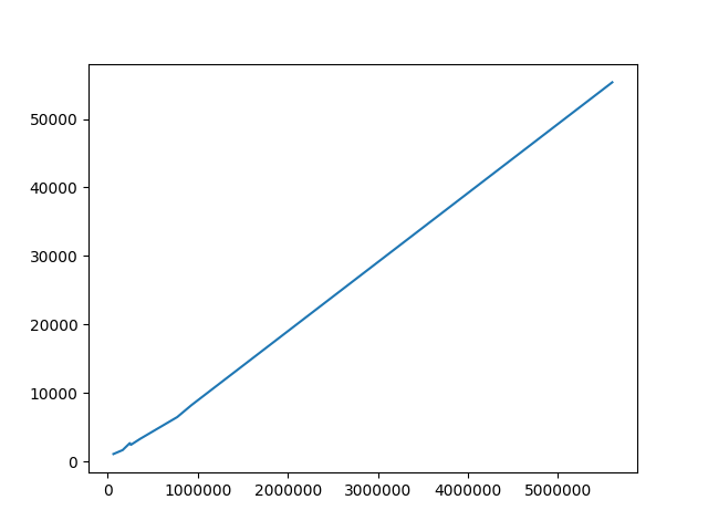
Which exactly says that time is linear and the hypothesis is proved.

7: Further Development

Processing images one by one in 2017 is boring. Here is a room for some parallelization. Also, we avoided RGB images for that reason. Of course, we can sort each channel separately, but it is way more interesting to process it in parallel.

If you liked this post and want to read about parallelization of this problem or say some criticism, or get new articles of this series/blog, you can send me an email.

Thank you for reading! Cheers.