Build Your Own Linear Regression: Implementations, Hyperparameters and their Optimizations
In this practice-driven post we will cover following topics:
- Linear Regression implementation in Python using Ordinary Least Squares method
- Linear Regression implementation in Python using Batch Gradient Descent method
- Their accuracy comparison to equivalent solutions from
sklearnlibrary - Hyperparameters study, experiments and finding best hyperparameters for the task
Hyperparameters are rarely mentioned, yet are particularly important because they affect both – accuracy and performance.
Sections
- Linear Regression: Implementation, Hyperparameters and their Optimizations
- Linear Regression: Ordinary Least Squares
- Linear Regression: Batch Gradient Descent
- Hyperparameters
- Conclusion
Linear Regression
Linear regression is kind of 'Hello, World!'
in machine learning field. I would assume that you are somewhat familiar with math behind it,
or at least you know what it does. In this post we will focus on conception, implementation
and experiments.
First of all, why is this regression linear? Simply because it represented by, literally, a linear equation:
$$ b_0 + w_1 * x_1 $$
which renders a staight line. Therefore regression is linear. You might assume that there exist a non-linear regression and you are right. This eqution is non-linear:
$$ b_0 + w_1 * x_1 + w_2 * x_1^2 $$
This equation will render not a straight line indeed because we introduced some non-linearity.
It is important to know that there are different kinds of regressions and linear is just one of them.
We will focus on linear regression because it is simple and interesting enough to implement and discuss.
Implementation
Before going any further, here is the link to GitHub with jupyter notebook which
you can clone and run on your local machine:
GitHub Jupyter Notebook Project
In this repository you can find all the code used to create this post, including helper functions, utilities, plots.
It is better to read this article and later look at the code in the notebook. I’ll omit some pieces such as imports and helpers for brevity.
Load Data
We will use diabetes
data from sklearn. Nothing prevents us from creating our own data, but we will
use sklearn to compare its accuracy to our accuracy so let’s stick to this lib
benefits.
Here we load the data and get relevant pieces to us. For now, we need only one feature from this multi-feature dataset.
full_data = datasets.load_diabetes()
one_feature = full_data.data[:, np.newaxis, 2]

x_training = one_feature[:-100]
y_training = full_data.target[:-100]
Plot
Let’s plot our training data <x, y>.
plt.scatter(x_training, y_training)
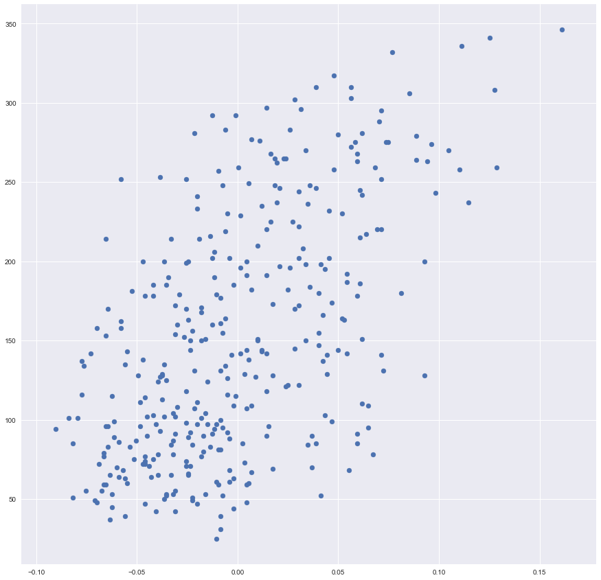
Data looks great!
However, one may see that we can not achieve a low value of a cost function because we have the big value of a variance here. In other words, our data is not looking like a line, it is more looking like an ellipsis.
Linear Regression: Ordinary Least Squares
In the implementation, I will not explain why it works in great details because it is a topic of two articles for each of the methods. If you are curious to understand the math behind it I can’t recommend Machine Learning course from Andrew Ng more. He explains these things just great and there is no need to fix what is not broken.
In statistics people tend to denote linear regression using the following notation $ y = b_0 + b_1 x $. While machine learning (read as more computer science-ish) crowd prefers to denote it as $ z = w_1 x + b $. Do not be confused. As you can see that this is the same thing, just a spelled differently.
We are computing bias b as:
$$ bias = \frac{\sum (x_i - mean(x))(y_i - mean(y))}{\sum (x_i - mean(x))^2} $$
Where $ \sum $ bounded from 1 to m. Weights w computed as:
$$ weight = mean(y) - (bias * mean(x)) $$
def ordinary_least_squares(x, y):
    '''
    Find weights for a hypothesis of the form:
        w*x + b
    using ordinary least squares method where
    w defined as b0, b as b1 by convention.

    Params:
        x: training data values
        y: training data lables

    Returns:
        hypothesis function
    '''
    xmean = np.mean(x)
    ymean = np.mean(y)

    m = len(x)

    numerator = 0
    denominator = 0

    for i in range(m):
        numerator += (x[i] - xmean) * (y[i] - ymean)
        denominator += (x[i] - xmean)**2

    b1 = numerator / denominator
    b0 = ymean - (b1 * xmean)

    # b1 and b0 are np arrays -> extract their actual values
    b = b0[0]
    w = b1[0]

    return lambda x: w*x + b
ordinary_least_squares is just a straight mapping from math to Python. First
we calculate means, next we compute sums, w and b.
💫 Successfully subscribed 💫
Get notified when post like this gets published.
Pavel Bazin writes about software engineering and engineering management. Some posts are highly technical dives with hands-on coding, others span into softs skills and carreer territory.
Create a Hypothesis
ordinary_least_squares returns a lambda function which represents a hypothesis,
so we can use it like an f(x) math function.
hypothesis = ordinary_least_squares(x_training, y_training)
If you are not familiar with higher order functions conception in programming
languages, here a short explanation what is happening: Our ordinary_least_squares
returns a function $ f(x) = wx + b $ , or talking in Python lambda x: w*x + b
where x is an argument. But where do we get w and b? Well, we get them
from the ordinary_least_squares, this stuff called a closure.
Make a Prediction
prediction = hypothesis(x_training)
prediction = prediction.reshape((342,))
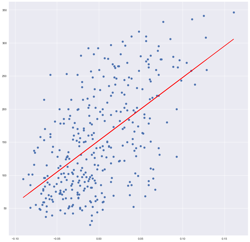
Plot Data and Linear Regression
Here is a huge advantage of working with a single feature data – this data can be projected onto 2D space, therefore visualized.
plt.scatter(x_training, y_training)
plt.plot(x_training, prediction, color='red')
By calling scatter function we are rendering our data, as we did in the beginning,
and calling a plot function we are rendering the line. Line’s x is a training
value and y is our prediction.

It seems that our Ordinary Least Square drew a nice line which indeed fits our data.
Verify
Let’s take LinearRegression from sklearn as an etalon implementation
and compare results with our custom solution.
model = linear_model.LinearRegression()
model.fit(x_training, y_training)
sk_prediction = model.predict(x_training)
Plot the result from sklearn library
plt.scatter(x_training, y_training)
plt.plot(x_training, sk_prediction, color='red')
Lines, predictions, seems to be identical. Let’s build an evaluator which can prove it numerically.
Implement an Evaluator
Mean squared error implementation:
def mean_squared_error_custom(truth, predicted):
    m = truth.shape[0]
    mse = (np.sum((predicted - truth)**2)) / (2*m)
    return mse
Mean squared error does exactly what it is named after. It takes an error, where an error is basically a distance between a predicted value and a truth, or actual, value and squares it. Next, we are summing up all the errors and take a mean value of them.
Squaring is needed because distance can be negative, but we are summing up all the errors, so our huge error can actually reduce the overall error which is a mistake. Something like mean modulo error will also work well.
Technically this one is a half mean squared error function. We half it for its nice derivative property.
Compare
Compare custom linear regression implementation and one from sklearn using
mean_squared_error_custom. So far plots are looking the same, but what about numbers?
print(mean_squared_error_custom(y_training, sk_prediction))
print(mean_squared_error_custom(y_training, prediction))
1965.39377764
1965.39377764
The result is the same, therefore implementation is perfectly correct.
Linear Regression: Batch Gradient Descent
First of all the Gradient Descent is an optimization method, one out of many but probably the most popular one.
Why do we need it? We really need it because it has a nice math properties which are crucial for modern machine learning, especially deep learning branch.
In our case gradient descent is simply better than ordinary least squares because it is faster and it is a more common tool. Here you can read more reasoning about it.
How it Works
Again, if you aren’t familiar with gradient descent conceptually, it is better to take Andrew Ng course for good comprehension. However here is the short explanation what is going on:
We want to minimize our overall loss. A loss is defined as a difference between predicted
values and truth values. To calculate loss we are computing predictions on our
training data and subtracting truth values from them: prediction - y. Next, we take a gradient of our cost function, which is its derivative, and calculate
its value with the loss, because it is what we want to eventually minimize.
The result of a gradient computation represents a slope of the cost function at a given point.
To optimize weights we must subtract the product
from learning rate and a gradient result from them. The learning rate is kind of a
filter which controls how big optimization steps are. For example, if learning
rate is 0.0001 and our gradient is -8.3124 our weight will change by 0.00083124,
if our learning rate is 1, then change in weight will be a negative identity of the gradient.
Why do we change sign? Because we want to move to global minima of our cost function,
and to do so we should modify our x axis value such that it will have as smallest
y as possible.
If you know math analysis this one should make sense, if it doesn’t make sense yet, I recommend reading this article by Eli Bendersky. If you don’t really know math analysis then you can try this one.
Implementation
Gradient descent is an iterative algorithm. Each iteration weights will be a little bit better than during the previous iteration.
We must use a method called a vectorization. This thing is crucial to modern machine learning computations and the main reason is performance. Instead of computing each weight for each feature of each training sample we abstract it away to tensor operations. There are lots of implementations of linear algebra operations and data containers for each language. And these operations are highly parallelizable because one operation doesn’t depend on any other.
Let’s prepare the data:
Xis a feature array with built-in biasoneswill act as a biasyground truth
x1 = full_data.data[:, np.newaxis, 1]
x1 = np.squeeze(np.asarray(x1[:-100]))

x2 = full_data.data[:, np.newaxis, 2]
x2 = np.squeeze(np.asarray(x2[:-100]))

ones = np.ones(len(x1))

X = np.array([ones, x1, x2]).T
y = full_data.target[:-100]
Here ones vector stays for a thing known as a bias. We can implement
the bias separately, or we can inject it into our training matrix.
Bias is full of ones because the reason that our hypothesis looks like this:
$$ h = x_1 w_1 + x_2 w_2 + … + x_m w_m $$
And if $ x_1 $ always equals to 1, then we have nothing but:
$$ h = x_1 w_1 + x_2 w_2 + … x_m-1 w_m-1 + bias $$
So it is just a matter of taste.
Here is the implementation of Batch Gradient Descent, where Batch stands for the fact that we are processing our data in batches, not on-by-one, but all at once.
def batch_gradient_descent(X, y, lrate, niter):
    weights = np.zeros(X.shape[1])

    history = []
    m = len(y)

    predict    = lambda x: np.dot(x, weights)
    derivative = lambda loss: (X.T.dot(loss)) / m

    for i in range(niter):
        hypothesis = predict(X)
        loss = hypothesis - y
        weights = weights - lrate * derivative(loss)

        if i % 50 == 0:
            history.append(mean_squared_error_custom(X.dot(weights), y))

    return predict, history
As with OLS, BGD returns a predictor which we can use as a function.
Why do we do
weights = weights - lrate * derivative(loss)instead ofweights -= lrate * derivative(loss)? Because-=won’t work. Python has object model and when you use operator-=actually you are usingobject.__iadd__(self, other). Sox += yis nothing butx = x.__iadd__(y), andx = x + yisx = x.__add__(y). Different libraries may use__iadd__and__add__differently, asnumpydoes.
Optimize Weights
predictor, history = batch_gradient_descent(X, y, 0.05, 50000)
Plot Training History
History was written by batch_gradient_descent each 50 iterations.
plt.plot(history)
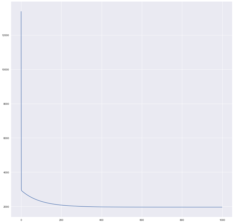
Seems that our training curve flattens out somewhere after ~400th the historical record, or ~20,000th iteration.
Make a Prediction and Get a Mean Squared Error
gds_predictions = X.dot(learned)
err = mean_squared_error_custom(gds_predictions, y)

print(err)
1963.4934
Validate
Validate the result of the custom BGD with running the same routine on the same data using sklearn library.
sk_reg = linear_model.LinearRegression()
sk_reg.fit(X, y)
sk_reg_pred = sk_reg.predict(X)

mean_squared_error(sk_prediction, y)
1965.3937
We can see that mean square error is kind of similar, but not the same. This happens because BGD has hyperparameters which can be tuned and edited, while OLS is a closed-math function which has no hyperparameters, therefore its output is always the same.
Hyperparameters
Perhaps the most interesting part of this article! Let’s observe how hyperparameters affect our algorithm in a most scientific way - empirically.
What hyperparameters are? The are some variable things which are set before actually optimizing the model’s weights. We encountered two numerical hyperparameters and one function.
Numerical:
- Learning Rate
- Number of Iterations
Function:
- Mean Squared Error
However, there are much more hyperparameters! What makes Linear Regression be linear regression? What is the difference between it and, say one layer neural network? Machine learning models are very much like LEGO. We can put together some pieces and fine-tune them. Putting one piece together we will end up with a linear regression. Put another pieces together we might end up with classification neural network. Here you can find more hyperparameters.
Let’s try to experiment with our hyperparameters.
batch_gradient_descent(X, y, lrate=???, niter=???)
In lrates we define various values for learning rate hyperparameter, and in niterations various values for a number of iterations.
The methodology looks as the following: we will run batch_gradient_descent with each possible combination of hyperparameters and compare them in multiple ways.
Let’s pick our hyperparameters to test. Generally, it is a good start to try .01
and we will take two 10 factor steps in each direction with an exception for the first item.
lrates = [.5, .1, .01, .001, .0001]
niterations = [25000, 50000, 150000]
test function iterates over each hyperparameter and put all the results
in a record list.
def test(X, y):
    record = []

    for niter in niterations:
        for lrate in lrates:
            start = time.time()
            weigths, records = batch_gradient_descent(X, y, lrate, niter)
            delta = time.time() - start
            record.append(dict(lrate=lrate, niter=niter, w=weigths, history=records, time=delta))

    return record
rec = test(X, y)
Plot
Lets plot all the batch_gradient_descent generated histories from test:
def plot_records(records):
    for record in records:
        label = 'lr: {0}, ni: {1}, t: {2}'.format(
          record["lrate"], record["niter"], record["time"])
        plt.plot(record['history'], label=label)
        plt.legend(bbox_to_anchor=(1.05, 1), loc=2, borderaxespad=0.)
plot_records(rec)
On this plot y axis stands for cost, and x axis stands for a number of iterations
or better to say a number of records. Little reminder here: why do we have 3,000
as a max value of x? This is because batch_gradient_descent make 1 record
in 50 iterations. So, to get iteration number we should multiply x by 50.
3,000 * 50 is 150,000 which is indeed our maximum value from niterations array.
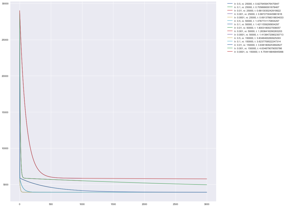
Hm, that doesn’t work well, isn’t it? Since we are doing experiments empirically it is OK to fail and look for a better visual representation!
Plot: Take 2
The first plot didn’t work out well so let’s plot each history record on the individual plot.
def plot_records(records):
    name_map = {0: 'A', 1: 'B', 2: 'C', 3: 'D', 4: 'E', 5: 'F', 6: 'G', 7: 'H', 8: 'I', 9: 'J', 10: 'K', 11: 'L', 12: 'M', 13: 'N', 14: 'O'}
    figure, plots = plt.subplots(5, 3)
    figure.tight_layout()
    plots = plots.flatten()
    for i, record in enumerate(records):
        time = "{0:.4f}".format(record['time'])
        label = 'lr: {0}, ni: {1}, t: {2}'.format(record["lrate"], record["niter"], time)
        plots[i].plot(record['history'], label=label)
        plots[i].legend(loc='upper right')
        plots[i].set_title(name_map[i])
plot_records(rec)
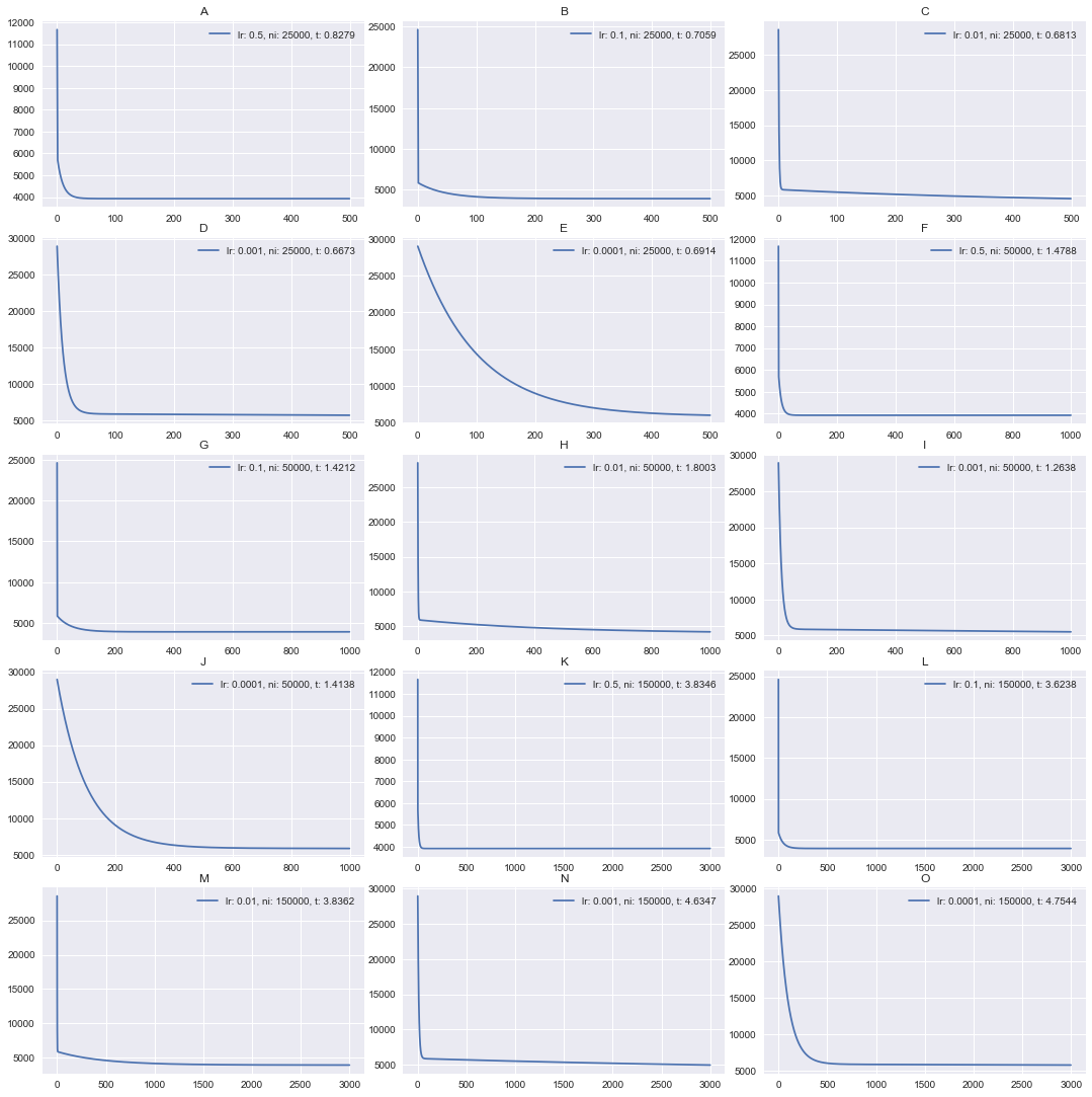
This is a good one. What do we see here? First of all, we can observe that some plots have almost 90-degree line, while some another is a smooth curve. While I visually like a curve on the plot, we may deduct that more angled plots are better.
They are better because their hyperparameters of batch_gradient_descent
converge much faster.
For example, look at [2, 2] plot (second line, second plot). It’s 5,000th
iteration, marked as 100 on the x axis, still has a cost value of ~14,500,
while plot [1, 2] already somewhere below 5,000. That’s a huge difference.
Numerical Data
Plot from above is good and easy to read, but let’s look at final numbers for
each batch_gradient_descent run.
First, prepare the data, sort it by time and print. Data will be sorted by time because I chosen this parameter as most important. Generally, we want to compute as fast as possible while the result is sufficiently good.
time_sorted_records = sorted(rec, key=lambda k: k['time'])
tab_data = time_sorted_records.copy()
for r in tab_data:
    r['cost'] = r['history'][-1]
    del r['history']
    del r['w']
print(tabulate.tabulate(time_sorted_records, headers={'lrate': 'lrate', 'niter': 'niter', 'time': 'elapsed time', 'cost': 'cost'}))
   lrate    niter    elapsed time     cost
 -------  -------  --------------  -------
  0.01      25000        0.298832  2299.74
  0.0001    25000        0.306833  3014.51
  0.1       25000        0.316224  1963.49
X 0.5       25000        0.333593  1963.47
  0.001     25000        0.33827   2846.12
  0.1       50000        0.584585  1963.47
  0.001     50000        0.587386  2755.94
  0.0001    50000        0.608037  2926.01
  0.01      50000        0.620816  2079.21
  0.5       50000        0.623807  1963.47
  0.5      150000        1.78622   1963.47
  0.1      150000        1.82313   1963.47
  0.0001   150000        1.83813   2884.86
  0.001    150000        1.84777   2478.86
  0.01     150000        1.86888   1965.21
We can see that cost 1963.47 can be considered to be the converged cost.
In our case, with the given data, learning rate of .5 converged after 25000 iterations, while learning rate of .0001 has a long way to go until convergence,
even after 150,000 iterations.
Lets find out how many iterations learning rate of .0001 needs to converge:
weights_t, records_t = batch_gradient_descent(X, y, 0.0001, 2000000)
print(records_t[-1])
2379.2350
Even after 2,000,000 iterations GBD with learning rate of .0001 converged to cost of 2379.2350.
In Finding of Optimal Hyperparameter Pair
Now we know that generally learning rate of .5 for this particular showed itself
very well, and we know that 1963.47 is the convergence value. If our first test
convergence value was found in 0.333593 seconds.
The question is: Can we get the same result, but faster?
lrates = [1.4, 1.2, 1, .8, .5]
niterations = [1000, 5000, 10000]

optimal_rec = test(X, y)

time_sorted_optimal_records = sorted(optimal_rec, key=lambda k: k['time'])
optimal_tab_data = time_sorted_optimal_records.copy()

for r in optimal_tab_data:
    r['cost'] = r['history'][-1]
    del r['history']
    del r['w']

print(tabulate.tabulate(optimal_tab_data, headers={'lrate': 'lrate', 'niter': 'niter', 'time': 'elapsed time', 'cost': 'cost'}))
  lrate    niter    elapsed time     cost
-------  -------  --------------  -------
    1.2     1000       0.0118332  1971.17
    0.8     1000       0.012208   2001.64
    1       1000       0.0124831  1980.58
    0.5     1000       0.0135529  2091.52
    1.4     1000       0.016505   1966.94
    0.5     5000       0.0545919  1963.5
 X  0.8     5000       0.0705771  1963.47
    1       5000       0.0712862  1963.47
    1.2     5000       0.0754931  1963.47
    1.4     5000       0.0930617  1963.47
    1      10000       0.119248   1963.47
    0.8    10000       0.133502   1963.47
    1.4    10000       0.140172   1963.47
    1.2    10000       0.168039   1963.47
    0.5    10000       0.20469    1963.47
Ok, seems that our winner is <0.8, 5000> pair. It converged in 0.0705771 seconds
which is 4.72 times faster than our previous best result.
Can We Do Better?
One may notice that so far the bigger value of a learning rate was the better one. So, let it be like 10 and we will converge in millisecond? Not quite. Let’s see it in action.
Repeat the test again with even higher learning rates:
lrates = [3, 2.5, 2, 1.5, .8]
niterations = [1000, 5000, 10000]

optimal_rec = test(X, y)
plot_records(optimal_rec)
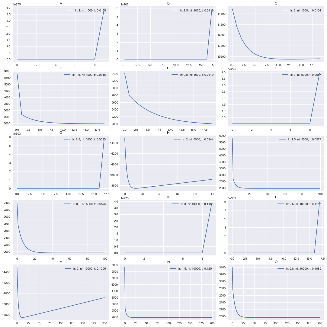
Did you expect that? It seems that learning rate >= 2 diverged. It can be
nicely seen on [3, 2] plot. We converge for a while, but after
that it start diverging, move in a reverse direction.
Conclusion
That is it. We implemented a linear regression in multiple ways using Python and numpy, validated our results properly, learned about hyperparameters and their optimizations.
💫 Successfully subscribed 💫
Liked the post? Get notified about the next one.
Pavel Bazin writes about software engineering and engineering management. Some posts are highly technical dives with hands-on coding, others span into softs skills and carreer territory.
As the last word, I would like to point out that never implement things yourself for production purpose unless you really, really know what you are doing and why. Even if your solution will be correct most likely it will be way slower than popular library equivalent.